Detecting smiles in pictures of my daughter: Building a machine learning model using Transfer Learning in Neural Networks

I recently created my first image classifier to categorize my daughter’s pictures into two-the ones where she is smiling and the other kind. It is a simple binary classification problem, but having very little data available and being new to it all i.e. motherhood and machine learning, I had to deal with a few challenges on the way. I thoroughly enjoyed working on this application though and would like to think that I learnt a thing or two in the process. It was very convenient to use a Kaggle kernel, to save myself the hassle of setting up my own local environment and to be able to get access to a GPU which was useful in training my model. In this article I will provide a step by step approach of creating this application, the challenges I faced and how I dealt with them. My work here is adapted from this great post which demonstrates how to classify dog and cat images, another binary classification problem.
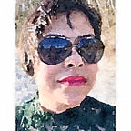
Just a side note: the internet can be a tricky place especially for children, hence to safeguard my daughter’s images I have converted the photos into watercolor pictures(using the app Waterlogue)before using them in this article. I used real images for training and testing the model though.

Why use transfer learning for this model? Instead of training the model from scratch for random initialization, we can make much faster progress if we download pre-trained weights and models and transfer that to our own model. One way of incorporating this method is by getting rid of the final output layer and creating our own unit that outputs the desired classification which in my case is the class smiling or not_smiling.The parameters of all the layers of the pre-trained model is considered frozen and you just need to train the parameters associated with your own final output layer.The main reason I am using transfer learning for my application is because by using pre-trained weights I can still aim to make a descent application with a small labeled dataset. In Andrew Ng’s very useful convolutional neural network course I had learned that you can have properties such as ‘trainable_weights’ and ‘freeze’ which allows you to modify the early layers accordingly. I have used trainable=0 for the pre-trained base model in-order to not recompute those activations every time I take an epoch or pass through the training set. You can also choose to freeze fewer layers and train the later layers in addition to the output layer. So depending on the amount of data you have the no. of layers frozen could be smaller and the no. of layers trained on top of the base model could be larger. For greater details on transfer learning I found the resources-Kaggle’s mini course on Deep Learning by Dan Becker and Andrew Ng’s Convolutional Neural Network course on Coursera very helpful.
I begin my application by importing all the packages I am going to use.
import cv2
import numpy as np
import pandas as pd
import matplotlib.pyplot as plt
%matplotlib inline
import gc
import os
import random
import seaborn as sns
sns.set()
from keras import backend as K
From the beginning, I decided to use Keras flow_from_directory() for the task. I was building my own dataset and could easily arrange my training data directory to contain subdirectories for each image class(a requisite for flow_from_directory() ). However there was a momentary hiccup when I tried creating the same subdirectories in my input folder in Kaggle. I tried several methods to create a folder structure under the input folder and try and upload images accordingly to no avail(newbie problems!).But you can do this very easily in Kaggle. In order to preserve your directory structure in your Kaggle dataset simply zip your files and upload the compressed file. You can see my folder structure in the adjacent image-one sub directory for each class. The classes in this case are smiling and not-smiling. Smiling contained all the pictures where my daughter is smiling and all the other images were put in the not-smiling folder. Since I had very little data and was trying to add to the data all the time while simultaneously coding, I decided to not create a separate validation folder containing the two classes. Instead my approach was to use train_test_split and reserve 20% for validation. This way I could just add my new images into the training classes and divide it later without worrying about accidentally modifying the percentage of the split.
train_smiling_dir='../input/smile-detection-dataset/smile-detection/train/smiling/'
train_not_smiling_dir='../input/smile-detection-dataset/smile-detection/train/not-smiling/'
test_dir='../input/smile-detection-dataset/smile-detection/test/'
I had around 400 pictures of my daughter which I could utilize to train my model. Initially I did face a class imbalance problem but I was able to quickly rectify that by taking more pictures of my daughter smiling-yeah I know! I took the easy way out. One of my immediate goals in the near future is to work on a custom weighted loss function to address this challenge.
image_size = 448I played around quite a bit with image_size trying 150,224 and finally settling for 448. This gave me the best results.
def create_img_name_list(path):
    listOfImages=[path+'{}'.format(i) for i in os.listdir(path)]
    return listOfImages
I created a function create_img_name_list that accepted a path and returned a list containing the names of the files in the directory.
#getting train and test images
train_smiling=create_img_name_list(train_smiling_dir)
train_not_smiling=create_img_name_list(train_not_smiling_dir)
test_imgs=create_img_name_list(test_dir)
train_imgs = train_smiling+train_not_smiling
random.shuffle(train_imgs)
del train_smiling
del train_not_smiling
gc.collect()
Using this function I create two lists for the two classes I am working with smiling and not_smiling . I also create a third list for the test images. The training images are then created by appending the smiling and not_smiling lists. I then randomly shuffled the training images which reorganizes the order of items. Without this there would be a bunch of smiling images followed by a bunch of not_smiling images which isn’t what we want. Hence shuffling here is important.
#Viewing some images in our train images
import matplotlib.image as mpimg
for key in list(train_imgs)[0:4]:
    img=mpimg.imread(key)
    imgplot=plt.imshow(img)
    plt.show()
I then viewed some of the images uploaded in the training set and noticed that the images are of different dimensions. This is mainly because in my pursuit of getting more data I went through all the videos I had of my daughter and took screenshots. In some cases I even had to crop out my husband or my face so as not to confuse the model. That resulted in images of all sorts of dimensions. Sorry about all the water color smudging! I do not know if it is evident from the adjacent images but these 2 images (Sample Image 1 and 2 from training set) are of very different sizes-the second one being larger than the first. No worries, that is where my next function read_and_process_image comes into play.

#Resizing images
nrows=image_size
ncolumns=image_size
channels=3
Prior to that I needed to decide on what would be the dimension of my images after processing. Since I am using colored images the number of channels used is 3.
#Reading and processing image to an acceptable format for our model
def read_and_process_image(train_images):
    """""
    Returns
    X:array of resized images
    y:array of labels
    """""
    X=[]
    y=[]
    for img in train_images:
       try:
        #for image in list_of_images:
        X.append(cv2.resize(cv2.imread(img,cv2.IMREAD_COLOR),(nrows,ncolumns),interpolation=cv2.INTER_CUBIC))
        #get the labels
        if 'not-smiling' in img:
            y.append(0)
        elif 'smiling' in img:
            y.append(1)
       except Exception as e:
        print(e)

    return X,y
The cv2 commands is used to resize the images. You can see below that both images are now of the same size.
If you remember, I had previously created lists with the full path of the images I would need to work with.Since my directory structure contained the folders ‘smiling’ and ‘not_smiling’ I have those texts in the names of the images belonging to the respective classes. I use that to create my y list by assigning 0 to images with ‘not-smiling’ in their names and 1 to images with ‘smiling’ in their names.
X,y=read_and_process_image(train_imgs)I call the read_and_process_image function to create the X and y arrays.Following are some of the pics after processing.

#Lets view some of the pics
plt.figure(figsize=(20,10))
columns = 5
for i in range(columns):
    plt.subplot(5 / columns + 1, columns, i + 1)
    plt.imshow(X[i])
Below I have plotted the frequency of each of the classes in my dataset. Ideally we want to train our model using an evenly balanced dataset so that the positive and negative training cases would contribute equally to the loss. 0 is for not-smiling and 1 represents the smiling class. I used seaborn for the data visualization.

import seaborn as sns
del train_imgs
gc.collect()#Convert list to numpy array
X = np.array(X)
y = np.array(y)sns.countplot(y)
plt.title('Labels for Smiling and Not-Smiling')
Next I split my training dataset into train and validation subsets. You will remember that I did not create a validation dataset up until this point because I was constantly adding images to my folders and did not want to make a mistake as to how many I added to training and how many to validation. I used sklearn’s train_test_split to assign 20% of my dataset for validation. Here is the code for the same.
#Lets split the data into train and test set
from sklearn.model_selection import train_test_split
X_train, X_val, y_train, y_val = train_test_split(X, y, test_size=0.20, random_state=2)
After creating the training and validation lists above, X and y are no longer required. I have also assigned a batch_size at this point which will be required for our model. In regards to batch_size I played around with values 8, 16 and 32 and saw that 32 gave the best results hence settled for that. At one point when I had only assigned 10% of the images to my validation subset, I was getting the error “local variable ‘logs’ referenced before assignment". This was because my validation dataset size was smaller than the batch size which I then quickly rectified by changing the percentage of images assigned to the validation set.
if K.image_data_format() == 'channels_first':
    X_train = X_train.reshape(X_train.shape[0], channels, nrows, ncolumns)
    #X_test = X_test.reshape(X_test.shape[0], channels, img_rows, img_cols)
    input_shape = (channels, nrows, ncolumns)
else:
    X_train = X_train.reshape(X_train.shape[0], nrows, ncolumns, channels)
    #X_test = X_test.reshape(X_test.shape[0], nrows, ncolumns, channels)
    input_shape = (nrows, ncolumns, channels)
I printed K.image_data_format() to check what was the value in my case and it showed ‘channels_last’. Hence the input_shape (nrows, ncolumns, channels) is being used in my scenario. According to this very helpful link which delves deeper into the subject-‘‘Channels last:Image data is represented in a three-dimensional array where the last channel represents the color channels, e.g. [rows][cols][channels].”
Next I used keras package for the pretrained InceptionResNetV2 model with imagenet as weights. Imagenet is a large image database used for image recognition. When the keras model is instantiated the weights are automatically downloaded(link) and the model is trained with the imagenet dataset. I did try the Resnet50 model too but got very poor results for my scenario(around 40% accuracy). Hence decided to stick with the InceptionResNetV2 model. The input_shape assigned here should be the same as the input_shape of your modified images i.e. shape of my images after I ran it through my function read_and_process_image.
from keras.applications import InceptionResNetV2conv_base = InceptionResNetV2(weights='imagenet', include_top=False, input_shape=input_shape)
Next I created a sequential model, added the pre-trained InceptionResNetV2 model and configured the top layer.
from keras import layers
from keras import modelsmodel = models.Sequential()
model.add(conv_base)
model.add(layers.Flatten())
model.add(layers.Dense(256, activation='relu'))
model.add(layers.Dense(1, activation='sigmoid'))
model.summary()
I then displayed the summary of the model which listed the no. of parameters configured.

Following this I printed the no. of trainable weights before and after I assign trainable=False to the pre-trained layer. Because I am using a pre-trained network, the weights are already learnt for the base layer, hence the choice to not train it again.
print('Number of trainable weights before freezing the conv base:', len(model.trainable_weights))
conv_base.trainable = False
print('Number of trainable weights after freezing the conv base:', len(model.trainable_weights))
The no. of weights before freezing is 492(mainly weights from conv_base) while after freezing the no. of trainable_weights are 4.
I then compiled the model and added the loss and optimizer parameters. Binary cross entropy is the loss function used for binary classification problems i.e. where there are two labeled classes, in my case smiling and not-smiling. “For each example, there should be a single floating-point value per prediction.”(link). You can read more about the adam optimization technique here.
model.compile(loss='binary_crossentropy', optimizer='adam',metrics=['acc'])Because I did not have enough data, I knew I needed to use image augmentation.Data augmentation is one of the techniques often used to improve the performance in computer vision systems. I used ImageDataGenerator which provides basic data augmentation methods such as rotation range and horizontal flip. I haven’t really played around with the hyperparameters in data augmentation-another one for the to-do list.
#Lets create the augmentation configuration
#This helps prevent overfitting, since we are using a small dataset
from keras.preprocessing.image import ImageDataGenerator
from keras.preprocessing.image import img_to_array, load_imgtrain_datagen = ImageDataGenerator(rescale=1./255,   #Scale the image between 0 and 1
                                    rotation_range=40,
                                    width_shift_range=0.2,
                                    height_shift_range=0.2,
                                    shear_range=0.2,
                                    zoom_range=0.2,
                                    horizontal_flip=True,
                                    fill_mode='nearest')val_datagen = ImageDataGenerator(rescale=1./255)  #We do not augment validation data. we only perform rescale#Create the image generators
train_generator = train_datagen.flow(X_train, y_train,batch_size=batch_size)
val_generator = val_datagen.flow(X_val, y_val, batch_size=batch_size)
#The training part
#Training for 25 epochs with about 9 steps per epoch
history = model.fit_generator(train_generator,
                              steps_per_epoch=ntrain // batch_size,
                              epochs=25,
                              validation_data=val_generator,
                              validation_steps=nval // batch_size,
                              verbose=1)

I got an accuracy of around 84% in 25 epochs. Considering the amount of data I have provided, I am pretty happy with the results.

Finally, I was ready to predict the images in my test dataset.
#Now lets predict on the images of the test set
X_test, y_test = read_and_process_image(test_imgs)
x = np.array(X_test)
test_datagen = ImageDataGenerator(rescale=1./255)i = 0
columns = 5
text_labels = []
plt.figure(figsize=(30,20))
for batch in test_datagen.flow(x, batch_size=1):
    pred = model.predict(batch)
    if pred > 0.5:
        text_labels.append('Smile detected!')
    else:
        text_labels.append('No smiles here.')
    plt.subplot(5 / columns + 1, columns, i + 1)
    plt.title(text_labels[i])
    imgplot = plt.imshow(batch[0])
    i += 1
    if i % 10 == 0:
        break
plt.show()

After running the model I get an accuracy in 9 out of 10 images. As of last night I also ran some of the modified watercolor images and voila! it worked too. Also a good idea to increase my training dataset this way. I have seen that images where there are multiple objects in the frame or my daughter is farther away are generally the ones failing. Over time I think I am going to add more data and make the classes more balanced, add a customized loss function and work further on hyperparameter optimization to fine-tune my model. I also plan to extend my application and make it a multi-class classifier, detect more emotions-wailing, hungry, sniffing nose etc. If nothing more comes off it, it would definitely be fun collecting that data! I would love to hear your suggestions if you have any in regards to ways I can improve this model to give better results.
Apart from these, one problem I keep facing is that my Kaggle dataset is unable to identify the kernel. Because of the growing nature of my data I keep removing, modifying and adding to my dataset and often times I face the dreaded FileNotFoundError. One way I am handling this now is by listing the directory contents of the input file.
print(os.listdir("../input"))In these scenarios I find that the directory contents are changed and I modify my path accordingly to read the files.
Thank you for staying with me and reading through my journey of coding my first fun neural network model.